On the inherent uncertainty of project tasks estimates

The accuracy of a project schedule depends on the accuracy of the individual activity (or task) duration estimates that go into it. Project managers  know this from (often bitter) experience.  Treatises such as the gospel according to PMBOK recognise this, and exhort project managers to estimate uncertainties and include them when reporting activity durations. However, the same books have little to say on how these uncertainties should be integrated into the project schedule in a meaningful way. Sure, well-established techniques such as PERT do incorporate probabilities into schedules via averaged or expected durations. But the resulting schedules are always treated as deterministic, with each task (and hence, the project)  having a definite completion date.  Schedules rarely, if ever, make explicit allowance for uncertainties.

In this post I look into the nature of uncertainty in project tasks – in particular I focus on the probability distribution of task durations. My approach is intuitive and somewhat naive. Having said that up front, I trust purists and pedants will bear with my somewhat loose use of terminology relating to probability theory.

Theory is good for theorists; practitioners prefer examples, so I’ll start with one. Consider an activity that you do regularly – such as getting ready in the morning.  Since you’ve done it so often, you have a pretty good idea how long it takes on average. Say it takes you an hour on average – from when you get out of bed to when you walk out of your front door. Clearly, on a particular day you could be super-quick and finish in 45 minutes, or even 40 minutes. However, there’s a lower limit to the early finish –  you can’t get ready in 0 minutes! Let’s say the lower limit is 30 minutes. On the other hand, there’s really no upper limit. On a bad day you could take a few hours.  Or if you slip in the shower and hurt your back, you could take a few days! So, in terms of probabilities, we have a 0% probability at a lower limit and also at infinity (since the probability of taking an infinite time to get to work is essentially zero). In between we’d expect the probability to hit a maximum at a lowish value of time (may be 50 minutes or so). Beyond the maximum, the probability would decay rapidly at first, then slowly becoming zero at an infinite time.

If we were to plot the probability of activity completion for this example as a function of time, it would look like the long-tailed function I’ve depicted in Figure 1 below. The distribution starts at a non-zero cutoff (corresponding to the minimum time for the activity); increases to a maximum (corresponding to the most probable time); and then falls off rapidly at first, then with a long, slowly decaying tail. The mean (or average) of the distribution is located to the right of the maximum because of the long tail. In the example,  (30 mins) is the minimum time for completion so the probability of finishing within 30 mins is 0%. There’s a 50% probability of completion within an hour (denoted by ), 80% probability of completion within 2 hours (denoted by ) and a 90% probability of completion in 3 hours (denoted by ). The large values for  and  compared to  are a consequence of the long tail. In the example, the tail –  which goes all the way to infinity – accounts for the remote possibility you may slip in the shower, hurt yourself  badly, and make it work very late (or may be not at all!).

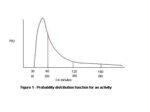
It turns out that many phenomena can be modeled by this kind of long-tailed distribution. Some of the better known long-tailed distributions include lognormal and power law distributions. A quick, informal review of project management literature revealed that lognormal distributions are more commonly used than power laws to model activity duration uncertainties. This may be because lognormal distributions have a finite mean and variance whereas power law distributions can have infinite values for both (see this presentation by Michael Mitzenmacher, for example). [An Aside:If you’re curious as to why infinities are possible in the latter, it is because power laws decay more slowly than lognormal distributions – i.e they have “fatter” tails, and hence enclose larger (even infinite) areas.]. In any case, regardless of the exact form of the distribution for activity durations, what’s important and non-controversial is the short cutoff, the peak and long, decaying tail. These characteristics are true of all probability distributions that describe activity durations.

There’s one immediate consequence of the long tail:   if you want to be really, really sure of completing any activity, you have to add a lot of “air” or  safety because there’s a chance that you may “slip in the shower” so to speak.  Hence, many activity estimators add large buffers to their estimates. Project managers who suffer the consequences of the resulting inaccurate schedule are thus victims of the tail.

Very few methodologies explicitly acknowledge  uncertainty in activity estimates, let alone present ways to deal with it. Those that do include  The Critical Chain Method, Monte Carlo Simulation and Evidence Based Scheduling.  The Critical Chain technique deals with uncertainty by slashing estimates to their values and consolidating safety or “air” into a single buffer, whereas the latter two techniques use simulations to generate expected durations (at appropriate confidence levels).  It would take me way past my self-imposed word limit to discuss these any further, but I urge you to follow the links listed above if you want to find out more.

(Note: Portions of this post are based on my article on the Critical Chain Method)