Building project knowledge – a social constructivist view

Introduction

Conventional approaches to knowledge management on projects focus on  the cognitive (or thought-related) and mechanical  aspects of knowledge creation and capture. There is alternate view, one which considers knowledge as being created through interactions between people who –  through their interactions –  develop mutually acceptable interpretations of theories and facts in ways that suit their particular needs. That is, project knowledge is socially constructed. If this is true, then project managers need to pay attention to the environmental and social factors that influence knowledge construction.  This is the position taken by Paul Jackson and Jane Klobas in their paper entitled, Building knowledge in projects: A practical application of social constructivism to information systems development, which presents a  knowledge creation / sharing process model based social constructivist theory. This article is a summary and review of the paper.

A social constructivist view of knowledge

Jackson and Klobas begin with the observation that engineering disciplines are founded on the belief that knowledge can be expressed in propositions that correspond to a reality which  is independent of human perception.  However, there is an alternate view that knowledge is not absolute, but relative – i.e.  it depends on the mental models and beliefs used to interpret facts, objects and events. A  relevant example is how a software product is viewed by business users and software developers. The former group may see an application in terms of its utility whereas the latter may see it as an instance of a particular technology. Such perception gaps can also occur within seemingly homogenous groups – such as teams comprised of software developers, for example. This can happen for a variety of reasons such as the differences in the experience and cultural backgrounds of those who make up the group. Social constructivism looks at how such gaps can be bridged.

The authors’ discussion relies on the work of Berger and Luckmann, who described how the gap between perceptions of different individuals can be overcome to create a socially constructed, shared reality. The phrase “socially constructed” implies that reality (as it pertains to a project, for example) is created via a common understanding of issues, followed by mutual agreement between all the players as to what comprises that reality. For me this view strikes a particular chord because of it is akin to the stated aims of dialogue mapping, a technique that I have described in several earlier posts (see this article for an example relevant to projects).

Knowledge in information systems development as a social construct

First up, the authors make the point that information systems development (ISD) projects are:

…intensive exercises in constructing social reality through process and data modeling. These models are informed with the particular world-view of systems designers and their use of particular formal representations. In ISD projects, this operational reality is new and explicitly constructed and becomes understood and accepted through negotiated agreement between participants from the two cultures of business and IT

Essentially, knowledge emerges  through interaction and discussion   as the project proceeds.  However, the methodologies used in design are typically founded on an engineering approach, which takes a positivist view rather than a social one. As the authors suggest,

Perhaps the social constructivist paradigm offers an insight into continuing failure, namely that what is happening in an ISD project is far more complex than the simple translation of a description of an external reality into instructions for a computer. It is the emergence and articulation of multiple, indeterminate, sometimes unconscious, sometimes ineffable realities and the negotiated achievement of a consensus of a new, agreed reality in an explicit form, such as a business or data model, which is amenable to computerization.

With this in mind, the authors aim to develop a model that addresses the shortcomings of the traditional, positivist view of knowledge in ISD projects. They do this by representing Berger and Luckmann’s theory of social constructivism in terms of a knowledge process model. They then identify management principles that map on to these processes. These principles form the basis of a survey which is used as an operational version of the process model. The operational model is then assessed by experts and tested by a project manager in a real-life project.

The knowledge creation/sharing process model

The process model that Jackson and Klobas describe is based on Berger and Luckmann’s work.

Figure 1: Knowledge creation/sharing model

The model  describes how personal knowledge is created – personal knowledge being what an individual knows. Personal knowledge is built up using mental models of the world – these models are frameworks that individuals use to make sense of the world.

According to the Jackson-Klobas process model, personal knowledge is built up through a number of process including:

Internalisation: The absorption of knowledge by an individual

Knowledge creation: The construction of new knowledge through repetitive performance of tasks (learning skills) or becoming aware of new ideas, ways of thinking or frameworks. The latter corresponds to learning concepts and theories, or even new ways of perceiving the world. These correspond to a change in subjective reality for the individual.

Externalisation: The representation and description of knowledge using speech or symbols so that it can be perceived and internalized by others. Think of this as explaining ideas or procedures to other individuals.

Objectivation: The creation of a shared constructs that represent a group’s understanding of the world. At this point, knowledge is objectified – and is perceived as having an existence independent of individuals.

Legitimation: The authorization of objectified knowledge as being “correct” or “standard.”

Reification: The process by which objective knowledge assumes a status that makes it difficult to change or challenge. A familiar example of reified knowledge is any procedure or process that is “hardened” into a system – “That’s just the way things are done around here,” is a common response when such processes are challenged.

The links depicted in the figure show the relationships between these processes.

Jackson and Klobas suggest that knowledge creation in ISD projects is a social process, which occurs through continual communication between the business and IT. Sure, there are other elements of knowledge creation – design, prototyping, development, learning new skills etc. – but these amount to nought unless they are discussed, argued, agreed on and communicated through social interactions. These interactions occur in the wider context of the organization, so it is reasonable to claim that the resulting knowledge takes on a form that mirrors the social environment of the organization.

Clearly, this model of knowledge creation is very different from the usual interpretation of knowledge having an independent reality, regardless of whether it is known to the group or not.

An operational model

The above is good theory, which makes for interesting, but academic, discussions. What about practice? Can the model be operationalised?  Jackson and Klobas describe an approach to creating to testing the utility (rather than the validity) of the model.  I discuss this in the following sections.

Knowledge sharing heuristics

To begin with, they surveyed the literature on knowledge management to identify knowledge sharing heuristics (i.e. experience-based techniques to enable knowledge sharing).  As an example, some of the heuristics associated with the externalization process were:

• We have standard documentation and modelling tools which make business requirements easy to understand
• Stakeholders and IS staff communicate regularly through direct face-to-face contact
• We use prototypes

The authors identified more than 130 heuristics. Each of these was matched with a process in the model. According to the authors, this matching process was simple: in most cases there was no doubt as to which process a heuristic should be attached to. This suggests that the model provides a natural way to organize the voluminous and complex body of research in knowledge creation and sharing. Why is this important? Well, because it suggests that the conceptual model (as illustrated in Fig. 1) can form the basis for a simple means to assess knowledge creation / sharing capabilities in their work environments, with the assurance that they have all relevant variables covered.

Validating the mapping

The validity of the matching was checked using twenty historical case studies of ISD projects. This worked as follows: explanations for what worked well and what didn’t were mapped against the model process areas (using the heuristics identified in the prior step). The aim was to answer the question:   “is there a relationship between project failure and problems in the respective knowledge processes or, conversely, between project success and the presence of positive indicators?”

One of the case studies the authors use is the well-known (and possibly over-analysed) failure of the automated dispatch system for the London Ambulance Service.  The paper has a succinct summary of the case study, which I reproduce below:

The London Ambulance Service (LAS) is the largest ambulance service in the world and provides accident and emergency and patient transport services to a resident population of nearly seven million people. Their ISD project was intended to produce an automated system for the dispatch of ambulances to emergencies. The existing manual system was poor, cumbersome, inefficient and relatively unreliable. The goal of the new system was to provide an efficient command and control process to overcome these deficiencies. Furthermore, the system was seen by management as an opportunity to resolve perceived issues in poor industrial relations, outmoded work practices and low resource utilization. A tender was let for development of system components including computer aided dispatch, automatic vehicle location, radio interfacing and mobile data terminals to update the status of any call-out. The tender was let to a company inexperienced in large systems delivery. Whilst the project had profound implications for work practices, personnel were hardly involved in the design of the system. Upon implementation, there were many errors in the software and infrastructure, which led to critical operational shortcomings such as the failure of calls to reach ambulances. The system lasted only a week before it was necessary to revert to the manual system.

Jackson and Klobas show how their conceptual model maps to knowledge-related factors that may have played a role in the failure project. For example, under the heading of personal knowledge, one can identify at least two potential factors: lack of involvement of end-users in design and selection of an inexperienced vendor. Further, the disconnect between management and employees suggests a couple of factors relating to reification: mutual negative perceptions and outmoded (but unchallenged) work practices.

From their validation, the authors suggest that the model provides a comprehensive framework that explains why these projects failed. That may be overstating the case – what’s cause and what’s effect is hard to tell, especially after the fact. Nonetheless, the model does seem to be able to capture many, if not all, knowledge-related gaps that could have played a role in these failures. Further, by looking at the heuristics mapped to each process, one might be able to suggest ways in which these deficiencies could have been addressed. For example, if externalization is a problem area one might suggest the use of prototypes or encourage face to face communication between IS and business personnel.

Survey-based tool

Encouraged by the above, the authors created a survey tool which was intended to evaluate knowledge creation/sharing effectiveness in project environments. In the tool, academic terms used in the model were translated into everyday language (for example, the term externalization was translated to knowledge sharing – see Fig 1 for translated terms). The tool asked project managers to evaluate their project environments against each knowledge creation process (or capability) on a scale of 1 to 10.   Based on inputs, it could recommend specific improvement strategies for capabilities that were scored low. The tool was evaluated by four project managers, who used it in their work environment over a period of 4-6 weeks. At the end of the period, they were interviewed and their responses were analysed using content analysis to match their experiences and requirements against the designed intent of the tool.  Unfortunately, the paper does not provide any details about the tool, so it’s difficult to say much more than paraphrase the authors comments.

Based on their evaluation, the authors conclude that the tool provides:

1. A common framework for project managers to discuss issues pertaining to knowledge creation and sharing.
2. A means to identify potential problems and what might be done to address them.

Field testing

One of the evaluators of the model tested the tool in the field. The tester was a project manager who wanted to identify knowledge creation/sharing deficiencies in his work environment, and ways in which these could be addressed.  He answered questions based on his own evaluation of knowledge sharing capabilities in his environment and then developed an improvement plan based on strategies suggested by the tool along with some of his own ideas.  The completed survey and plan were returned to the researchers.

Use of the tool revealed the following knowledge creation/sharing deficiencies in the project manager’s environment:

1. Inadequate personal knowledge.
2. Ineffective externalization
3. Inadequate standardization (objectivation)

Strategies suggested by the tool include:

1. An internet portal to promote knowledge capture and sharing. This included discussion forums, areas to capture and discuss best practices etc.
2. Role playing workshops to reveal how processes worked in practice (i.e. surface tacit knowledge).

Based on the above, the authors suggest that:

1. Technology can be used to promote support knowledge sharing and standardization, not just storage.
2. Interventions that make tacit knowledge explicit can be helpful.
3. As a side benefit, they note that the survey has raised consciousness about knowledge creation/sharing within the team.

Reflections and Conclusions

In my opinion, the value of the paper lies not in the model or the survey tool, but the conceptual framework that underpins them – namely, the idea knowledge depends on, and is shaped by, the social environment in which it evolves. Perhaps an example might help clarify what this means. Consider an organisation that decides to implement project management “best practices” as described by <fill in any of the popular methodologies here>. The wrong way to do this would be to implement practices wholesale, without regard to organizational culture, norms and pre-existing practices. Such an approach is unlikely to lead to the imposed practices taking root in the organisation. On the other hand, an approach that picks the practices that are useful and tailors these to organizational needs, constraints and culture is likely to meet with more success. The second approach works because it attempts to bridge gap between the “ideal best practice” and social reality in the organisation. It encourages employees to adapt practices in ways that make sense in the context of the organization. This invariably involves modifying practices, sometimes substantially, creating new (socially constructed!) knowledge in the bargain.

Another interesting point the authors make is that several knowledge sharing heuristics (130, I think the number was) could be classified unambiguously under one of the processes in the model. This suggests that the model is a reasonable view of the knowledge creation/sharing process. If one accepts this conclusion, then the model does indeed provide a common framework for discussing issues relating knowledge creation in project environments. Further, the associated heuristics can help identify processes that don’t work well.

I’m unable to judge the usefulness of the survey-based tool developed by the authors because they do not provide much detail about it in the paper. However, that isn’t really an issue;  the field of project management has too many “tools and techniques” anyway.  The key message of the paper, in my opinion, is the that every project has a unique context, and that the techniques used by others have to be interpreted and applied in ways that are meaningful in the context of the particular project. The paper is an excellent counterpoint to the methodology-oriented practice of knowledge management in projects; it should be required reading for methodologists and  project managers who believe that things need to be done by The Book, regardless of social or organizational context.

Monte Carlo simulation of multiple project tasks – three examples and some general comments

Introduction

In my previous post I  demonstrated the use of a Monte Carlo technique in simulating  a single project task with completion times  described by a triangular distribution.  My aim in that article was to:  a) describe a Monte Carlo simulation procedure in enough detail for someone interested to be able to reproduce the calculations and b) show that it gives sensible results in a situation where the answer is known.  Now it’s time to take things further.  In this post, I present simulations for two tasks chained together in various ways.  We shall see that, even with this small increase in complexity (from one task to two), the results obtained can be surprising.  Specifically, small changes in inter-task dependencies can have a huge effect on the overall (two-task) completion time distribution. Although, this is something that that most project managers have experienced in real life, it is rarely taken in to account by traditional scheduling techniques. As we shall see, Monte Carlo techniques predict such effects as a matter of course.

Background

The three simulations discussed here are built on the example that I used in my previous article, so it’s worth spending a few lines for a brief recap of that example.  The task simulated in the example was assumed to be described by a triangular distribution with  minimum completion time () of 2  hours,   most likely completion time () of 4 hours and   a maximum completion time () of 8 hours.   The resulting triangular probability distribution function (PDF),  –  which gives the probability of completing the task at time t – is shown in Figure 1.

Figure 1 - PDF for triangular distribution (tmin=2, tml=4, tmax=8)

Figure 2 depicts the associated cumulative distribution function (CDF),   which gives the probability that a task will be completed by time t (as opposed to the PDF which specifies the probability of completion at time t). The value of the CDF at t=8 is 1 because the task must finish within 8 hrs.

Figure 2 - PDF for triangular distribution (tmin=2, tml=4, tmax=6)

The equations describing the PDF and CDF are listed in equations 4-7 of my previous article.  I won’t rehash them here as they don’t add anything new  to the discussion – please see the article for all the gory algebraic details and formulas.   Now, with that background, we’re ready to move on to the examples.

Two tasks in series with no inter-task delay

As a first example, let’s look at two tasks that have to be performed sequentially – i.e. the second task starts as soon as the first one is completed. To simplify things, we’ll also assume that they have identical (triangular) distributions as described earlier and shown in Figure 1  (excepting , of course,  that the distribution is shifted to the right for the second task  – since it starts after the first one finishes).  We’ll also  assume that the second task begins right after the first one is completed (no inter-task delay) – yes, this is unrealistic, but bear with me.  The simulation algorithm for the  combined tasks is very similar to the one for a single task (described in detail in my previous post). Here’s the procedure:

1. For each of the two tasks, generate a set of N random numbers. Each random number generated corresponds to the cumulative probability of completion for a single task on that particular run.
2. For each random number generated, find the time corresponding to the cumulative probability by solving equation 6 or 7 in my previous post.
3. Step 2 gives N sets of completion times. Each set has two completion times – one for each tasks.
4. Add up the two numbers in each set to yield the comple. The resulting set corresponds to N simulation runs for the combined task.

I then divided the time interval from t=4 hours  (min possible completion time for both tasks) to t=16 hours (max possible completion time for both tasks) into bins of 0.25 hrs each, and then assigned each combined completion time to the appropriate bin. For example, if the predicted completion time for a particular run was 9.806532 hrs, it was assigned to the bin corresponding to 0.975 hrs.  The resulting histogram is shown in Figure 3 below (click on image to view the full-size graphic).

Figure 3 - Frequency histogram for tasks in series with no inter-task delay

[An aside:  compare the histogram in Figure 3 to the one for a single task (Figure 1):  the distribution for the single task is distinctly asymmetric (the peak is not at the centre of the distribution) whereas the two task histogram is nearly symmetric.  This surprising result is a consequence of the Central Limit Theorem (CLT) – which states that the sum of many identical distributions tends to resemble the Normal (Bell-shaped) distribution, regardless of the shape of the individual distributions.   Note that the CLT holds even though the two task distributions are shifted relative to each other – i.e. the second task begins after the first one is completed.]

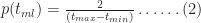
The simulation also enables us to compute the cumulative probability of completion for the combined tasks (the CDF). This value of the cumulative probability at a particular bin equals the sum of the number of simulations runs in every bin up to (and including) the bin in question, divided by the total number of simulation runs. In mathematical terms this is:

where   is the cumulative probability at the time corresponding to the  th  bin, , the number of simulation runs in the th  bin and    the total number of simulation runs. Note that this formula is an approximate one because time is treated as a constant within each bin. The approximation can be improved by making the bins smaller (and hence increasing the number of bins).

The resulting cumulative probability function is shown in Figure 4. This allows us to answer questions such as:  “What is the probability that the tasks will be completed within 10 days?”. Answer:  .698, or approximately 70%. (Note:  I obtained this number by interpolating between values obtained from equation (1), but this level of precision is uncalled for, particularly because the formula is an approximate one)

Figure 4 - CDF for tasks in series with no inter-task delay

Many project scheduling techniques compute average completion times for component tasks and then add them up to get the expected completion time for the combined task. In the present case the average works out to 9.33 hrs (twice the average for a single task). However, we see from the CDF that there is a significant probability (.43) that we will not finish by this time – and this in a “best-case ” situation where the second task starts immediately after the first one finishes!

[An aside: If one applies the  well-known PERT formula   to each of the tasks, one gets an expected completion time  of 8.66 hrs for the combined task.  From the CDF one can show that there is a  probability of non-completion of 57%  by t=8.66 hours (see Figure 4) – i.e. there’s a greater than even chance of not finishing by this time!]

As interesting as this case is, it is somewhat unrealistic because successor tasks seldom start the instant the predecessor is completed. More often than not, there is a cut-off time before which the successor cannot start – even if there are no explicit dependencies between the two tasks.  This observation is a perfect segue into my next example, which is…

Two tasks in series with a fixed earliest start for the successor

Now we’ll introduce a slight complication: let’s assume, as before, that the two tasks are done one after the other but that the earliest the second task can start is at hours  (as measured from the start of the first task). So, if the first task finishes within 6 hours, there will be a delay between its completion and the start of the second task. However, if the first task takes longer than 6 hours to finish, the second task will start soon after the first one finishes.  The simulation procedure is the same as described in the previous section excepting for the last step – the completion time for the combined task is given by:

, for t   6 hrs and , for t < 6 hrs

I divided the time interval from t=4hrs to t=20 hrs into bins of 0.25 hr duration (much as I did before) and then assigned each combined completion time to the appropriate bin. The resulting histogram is shown in Figure 5.

Figure 5 - Frequency histogram for tasks in series with inter-task delay

Comparing Figure 5 to Figure 3, we see that the earliest possible finish time now increases from 4 hrs to 8 hrs. This is no surprise, as we built this in to our assumption.  Further, as one might expect, the distribution is distinctly asymmetric – with a minimum completion time of 8 hrs, a most likely time between 10 and 11 hrs and a maximum completion time of about 15 hrs.

Figure 6 shows the cumulative probability of completion for this case.

Figure 6 - CDF for tasks in series with inter-task delay

Because of the delay condition, it is impossible to calculate the average completion from the formulas for the triangular distribution – we have to obtain it from the simulation.  The average can be calculated from the simulation adding up all completion times and dividing by the total number of simulations, . In mathematical terms this is:

where is the average time,    the completion time for the th simulation run and    the total number of simulation runs.

This procedure gave me a value of about 10.8  hrs for the average.  From the CDF in Figure 6 one sees that the probability that the combined task will finish by this time is only 0.60 – i.e. there’s only a 60% chance that the task will finish by this time.  Any naïve estimation of time would do just as badly unless, of course, one is overly pessimistic and assumes a completion time of 15 – 16 hrs.

From the above it should be evident that the simulation allows one to associate an uncertainty (or probability) with every estimate. If management imposes a time limit of 10 hours,  the project manager can refer to the CDF in Figure 6 and figure out the probability of completing the task by that time (there’s a 40 % chance of completion by 10 hrs).  Of course, the reliability of the numbers depend on how good the distribution is. But  the assumptions that have gone into the model are known –  the optimistic, most likely and pessimistic times and the form of the distribution – and these can be refined as one gains experience.

Two tasks in parallel

My final example is the case of two identical tasks performed in parallel. As above, I’ll assume the uncertainty in each task is characterized by a triangular distribution with ,   and  of 2, 4 and 8 hours respectively. The simulation procedure for this case is the same as in the first example, excepting the last step. Assuming the simulated completion times for the individual tasks are and , the completion time for the combined tasks is given by the greater of the two – i.e. the combined completion time is given by .

To plot the histogram shown in Figure 7 , I divided the interval from t=2 hrs to t=8 hrs into bins of 0.25 hr duration each (Warning: Note the difference in the time axis scale  from Figures 3 and 5!).

Figure 7 - Frequency histogram for tasks in parallel

It is interesting to compare the above  histogram with that for an individual task with the same parameters (i.e. the example that was used in my previous post). Figure 8 shows the histograms for the two examples on the same plot (the combined task in red and the single task in blue). As one might expect, the histogram for the combined task is shifted to the right, a consequence of the nonlinear condition on the completion time.

Figure 8 - Histograms for tasks in parallel (red) and single task (blue)

What about the average? I calculated the average as before, by using equation (2) from the previous section. This gives an average of 5.38 hrs (compared to 4.67 hrs for either task, taken individually).   Note that the method to calculate the average is the same regardless of the form of the distribution. On the other hand,  computing the average from the equations would be a complicated affair, involving a stiff dose of algebra with an optional  sprinkling of  calculus.  Even worse – the calculations would vary from distribution to distribution. There’s no question that simulations are much easier.

The CDF for the overall completion time is also computed easily using equation (1). The resulting plot is shown in Figure 9  (Note the difference in the time axis scale  from Figures  4 and 6!). There are no surprises here – excepting how easy it is to calculate once the simulation is done.

Figure 9 - CDF for tasks in parallel

Let’s see what time corresponds to a 90% certainty of completion. A rough estimate for this number can be obtained from Figure 9 – just find the value of t (on the x axis) corresponding to a cumulative probability of 0.9 (on the y axis).  This is the graphical equivalent of solving the CDF for time, given the cumulative probability is 0.9. From Figure 9, we get a time of approximately 6.7 hrs. [Note: we could get a more accurate number by fitting the points obtained from equation (1) to a curve and then calculating the time corresponding to ]. The interesting thing is that the 90% certain completion time is not too different from that of a single task (as calculated from equation 7 of my previous post) – which works out to 6.45 hrs.

Comparing the two histograms in Figure 8, we expect the biggest differences in cumulative probability to occur at about the t=4 hour mark, because by that time the probability for the individual task has peaked whereas that for the combined task is yet to peak. Let’s see if this is so: from Figure 8, the cumulative probability for t=4  hrs is about .15 and from the CDF for the triangular distribution (equation 6 from my previous post), the cumulative probability at t=4 hours  (which is the most likely time) is .333 – double that of the combined task.  This, again, isn’t too surprising (once one has Figure 8 on hand). The really nice thing is that we are able to attach uncertainties to all our estimates.

Conclusion

Although the examples discussed above are simple – two identical tasks with uncertainties described by a triangular distribution – they serve to illustrate some of the non-intuitive outcomes when tasks have dependencies.   It is also worth noting that although the distribution for the individual tasks is known, the only straightforward way to obtain the distributions for the combined tasks (figures 3, 5 and 7) is through simulations. So, even these simple examples are a good demonstration of the utility of Monte Carlo techniques. Of course, real projects are way more complicated, with diverse tasks distributed in many different ways.   To simplify simulations in such cases,  one could  perform  coarse-grained simulations on a small number of high-level tasks,  each consisting of a number of  low-level, atomic tasks. The high-level tasks could be constructed in such a way as to focus attention on areas of greatest complexity, and hence greatest uncertainty.

As I have mentioned several times in this article and the previous one: simulation results are only as good as the distributions on which they are based. This begs the question: how do we know what’s an appropriate distribution for a given situation? There’s no one-size-fits-all answer to this question. However, for project tasks there are some general considerations that apply. These are:

1. There is a minimum time () before which a task cannot cannot be completed.
2. The probability will increase from 0 at to a maximum at a “most likely” completion time, . This holds true for most atomic tasks – but may be not for composite tasks which consist of many smaller tasks.
3. The probability decreases as time increases beyond ,  falling to 0 at a time much larger than .   This is simply another way of saying that the distribution has a long (but not necessarily infinite!) tail.

Asymmetric triangular distributions (such as the one used in my examples) are the simplest distributions that satisfy these conditions. Furthermore, a three point estimate is enought to specify a triangular distribution completely – i.e. given a three point estimate there is only one triangular distribution that can be fitted to it. That said, there are several other distributions that can be used; of particular relevance are certain long-tailed distributions.

Finally, I should mention that I make no claims about the efficiency or accuracy of the method presented here:  it should be seen  as  a demonstration rather than a definitive technique.  The many commercial Monte Carlo tools available in the market probably offer far more comprehensive, sophisticated and reliable algorithms (Note:  I ‘ve never used any of them, so I can’t make any recommendations!).  That said, it is always helpful to know the principles behind such tools,  if for no other reason than to understand how they work and, more important,  how to use them correctly.  The material discussed in this and the previous article came out of my efforts to develop an understanding Monte Carlo techniques and how they can be applied to various aspects of project management (they can also be applied to cost estimation, for example).  Over the last few weeks  I’ve spent many enjoyable evenings developing and running these simulations, and learning from them.  I’ll  leave it here with the hope that you find my articles helpful in your own explorations of the wonderful world of Monte Carlo simulations.

An introduction to Monte Carlo simulation of project tasks

Introduction

In an essay on the uncertainty of project task estimates,  I  described how a task estimate corresponds to a  probability distribution.  Put simply, a task estimate is actually a range of possible completion times, each with a probability of occurrence specified by a distribution.   If one knows the distribution,  it is possible to answer questions  such as:  “What is the probability that the task will be completed within x days?”

The reliability of such predictions depends on how faithfully the distribution captures the actual  spread of task durations –  and therein lie at least a couple of problems.   First,  the probability distributions for task durations are generally hard to characterise because of the lack of reliable data (estimators are not very good at estimating, and historical data is usually not available).  Second,  many realistic distributions have complicated mathematical forms which can be hard to characterise and manipulate.

These problems are compounded by the fact that projects consist of several tasks, each one with its own duration estimate and  (possibly complicated) distribution.  The first issue is usually addressed by fitting distributions to  point estimates (such as optimistic, pessimistic and most likely times as in PERT)  and then  refining these estimates and distributions as one gains experience.  The second issue can be tackled by Monte Carlo techniques, which involve  simulating the task a number of times  (using an appropriate distribution) and then calculating expected completion times based on the results.   My aim in this post  is to present an  example-based  introduction to Monte Carlo simulation of project task durations.

Although my aim is to keep things reasonably simple (not too much beyond high-school maths and a basic understanding of probability), I’ll be covering a fair bit of ground. Given this,  I’d best to start with a brief description of my approach so that my readers know what coming.

Monte Carlo simulation is an umbrella term that  covers a range of approaches that use random sampling to simulate events that are described by known probability distributions.  The first task then, is to specify the probability distribution. However, as mentioned earlier, this is generally unknown for task durations. For simplicity, I’ll assume that task duration uncertainty can be described accurately using a triangular probability distribution – a distribution that is particularly easy to handle from the mathematical point of view. The advantage of using the triangular distribution is that simulation results can be validated easily. 

Using the triangular distribution isn’t a limitation because the method I describe can be applied to arbitrarily shaped distributions. More important, the technique can be used to simulate what happens when multiple tasks are strung together as in a project schedule (I’ll cover this in a future post).  Finally, I’ll demonstrate a Monte Carlo simulation method as applied to a single task described by a triangular distribution. Although a simulation is overkill in this case (because questions regarding durations can be answered exactly without using a simulation),  the example serves to illustrate the steps involved in simulating more complex cases – such as those comprising of more than one task and/or involving more complicated distributions.

So, without further ado, let me begin the journey by describing the triangular distribution.

The triangular distribution

Let’s assume that there’s a project task that needs doing, and the person who is going to do it reckons it will take between 2 and 8 hours to complete it, with a most likely completion time of 4 hours. How the estimator comes up with these numbers isn’t important at this stage – maybe there’s some guesswork, maybe some padding or maybe it is really based on experience (as it should be).  What’s important is that we have three numbers corresponding to a minimum, most likely and maximum time.  To keep the discussion general, we’ll call these , and respectively, (we’ll get back to our estimator’s specific numbers later).

Now, what about the probabilities associated with each of these times?

Since and correspond to the minimum and maximum times,  the probability associated with these is zero. Why?  Because if it wasn’t zero, then there would be a non-zero probability of completion for a time less than or greater than – which isn’t possible [Note: this is a consequence of the assumption that the probability varies continuously –  so if it takes on non-zero value, ,  at then it must take on a value slightly less than – but greater than 0 –  at  slightly smaller than  ] .   As far as  the most likely time,  ,  is concerned:  by definition, the probability attains its highest value at time .    So, assuming the probability can be described by a triangular function, the distribution must have the form shown in Figure 1 below.

Figure 1: Triangular Distribution

For the simulation, we need to know the equation describing the above distribution.  Although Wikipedia will tell us the answer in a mouse-click, it is instructive to figure it out for ourselves. First, note that the area under the triangle must be equal to  1 because the task must finish at some time between and .   As a consequence we have:

where  is the probability corresponding to time .  With a bit of rearranging we get,

To derive the probability for any time lying between and , we note that:

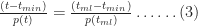
This is a consequence of the fact that the ratios on either side of equation (3)  are  equal to the slope of the line joining the points and .

Figure 2

Substituting (2) in (3) and simplifying a bit, we obtain:

for

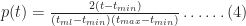
In a similar fashion one can show that the probability for times lying between and is given by:

for

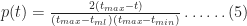
Equations 4 and 5 together describe the probability distribution function (or PDF)  for all times between and .

Another quantity of  interest is the cumulative distribution function (or CDF) which is the probability, ,  that the task is completed by a time . To reiterate, the PDF, , is the probability of the task finishing at time whereas the CDF, , is the probability of the task completing by time . The CDF, ,  is essentially a sum of all probabilities between and . For this is the area under the triangle with apexes at   (, 0), (t, 0) and (t, p(t)).  Using the formula for the area of a triangle (1/2 base times height) and equation (4) we get:

for

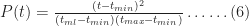
Noting that for , the area under the curve equals the total area minus the area enclosed by the triangle with base between t and , we have:

for

As expected,   starts out with a value 0 at and then increases monotonically, attaining a value of 1 at .

To end this section let's plug in the numbers quoted by our estimator at the start of this section: , and .  The resulting PDF and CDF are shown in figures 3 and 4.

Figure 4 – Triangular CDF (tmin=2, tml=4, tmax=8)

Monte Carlo Simulation of  a Single Task

OK, so now we get to the business end of this essay – the simulation.  I’ll first outline the simulation procedure and  then discuss results for the case of  the task described in the previous section (triangular distribution with , and ).  Note that I used TK Solver – a mathematical package created by Universal Technical Systems – to do the simulations. TK Solver has built-in backsolving capability which is extremely helpful for solving some of the equations that come up in the simulation calculations. One could use Excel too, but my spreadsheet skills are not up to it :-(.

So, here’s my  simulation procedure:

1. Generate a random number between 0 and 1.  Treat this number as the cumulative probability,  for the simulation run. [Technical Note:  I used the random number generator that comes with the TK Solver package (the algorithm used by the generator is described here). Excel’s random number generator is even better.]
2. Find the time, ,  corresponding to by solving equations (6) or (7) for . The resulting value of is the time taken to complete the task. [Technical Note: Solving equation (6) or (7) for isn’t straightforward because appears in several places in the equations. One has two options to solve for a) Use numerical techniques such as the bisection or Newton-Raphson method or b) use the backsolve (goal seek) functionality in Excel or other mathematical packages. I used the backsolving capability of TK Solver to obtain t for each random value of P generated. TK Solver backsolves equations automatically –  no fiddling around with numerical methods – which makes it an attractive option for these kinds of calculations.]
3. Repeat steps (1) and (2)  N times, where N is a “sufficiently large” number – say 10,000.

I did the calculations for using the triangular distribution with parameters , and . This gave me 10,000 values of and .

As an example of a simulation run proceeds, here’s the data from my first simulation run: the random number generator returned 0.490474700804856 (call it 0.4905). This is the value of . The time corresponding to this cumulative probability is obtained by solving equation (7) numerically for . This gave (call it 4.503) as shown in Figure 5. This is the completion time for the first run.

Figure 5

After completing 10,000 simulation runs, I sorted these into bins corresponding to time intervals of .25 hrs, starting from =2hrs through to =8 hrs. The resulting histogram is shown in Figure 6. Each bar corresponds to the number of simulation runs that fall within that time interval.

Figure 6: Distribution of simulation runs

As one might expect, this looks like the triangular distribution shown in Figure 4. There is a difference though: Figure 4 plots probability as a continuous function of time  whereas Figure 6 plots the number of simulation runs as a step function of time. To convince ourselves that the two are really the same, lets look at the cumulative probability at   – i.e the probability that the task will be completed within 4 hrs. From equation 6 we get .  The corresponding number from the simulation is simply the number of simulation runs that had a completion time less than or equal to 4 hrs,  divided by the total number of simulation runs. For my simulation this comes out to be 0.3383. The agreement’s not perfect, but is convincing enough. Just to be sure, I performed the simulation a number of times – generating several sets of random numbers – and took the average of the predicted . The agreement between theory and simulation improved, as expected.

Wrap up

A limitation of the triangular distribution is that it imposes an upper cut-off at . Long-tailed distributions may therefore be more realistic. In the end, though, the form distribution is neither here nor there because the technique can be applied to any distribution. The real question is:  how do we obtain reliable distributions for our estimates? There’s no easy answer to this one, but one can start with three point estimates (as in PERT) and then fit these to a triangular (or more complicated) distribution.  Although it is best if one  has historical data, in the absence this one can always start with reasonable guesses. The point is to refine these through experience.

Another point worth mentioning is that simulations can be done at a level higher than that of an indivdual task. In their brilliant book – Waltzing With Bears: Managing Risk on Software Projects – De Marco and Lister demonstrate the use of Monte Carlo methods to simulate various aspects of project – velocity, time, cost etc. – at the project level (as opposed to the task level). I believe it is better to perform simulations at the lowest possible level (although it is a lot more work) – the main reason being that it is easier, and less error-prone, to estimate individual tasks than entire projects. Nevertheless, high level simulations can be very useful if one has reliable data to base these on.

I would be remiss if I didn’t mention some of the various Monte Carlo packages available in the market. I’ve never used any of these, but by all accounts they’re pretty good: see this commercial package or this one, for example. Both products use random number generators and sampling techniques that are far more sophisticated than the simple ones I’ve used in my example.

Finally, I have to admit that the example described in this post is a very complicated way of demonstrating the obvious – I started out with the triangular distribution and then got back the triangular distribution via simulation. My point, however, was to illustrate the method and show that it yields expected results in a situation where the answer is known. In a future post I’ll apply the method to more complex situations- for example, multiple tasks in series and parallel, with some dependency rules thrown in for good measure.  Although, I’ll use the triangular distribution for individual tasks, the results will be far from obvious: simulation methods really start to shine as complexity increases. But all that will have to wait for later. For now, I hope my example has helped illustrate how Monte Carlo methods can be used to simulate project tasks.

Note added on 21 Sept 2009:

Follow-up to this article published here.

Note added on 14 Dec 2009:

See this post for a Monte Carlo simulation of correlated project tasks.