A gentle introduction to logistic regression and lasso regularisation using R
In this day and age of artificial intelligence and deep learning, it is easy to forget that simple algorithms can work well for a surprisingly large range of practical business problems. And the simplest place to start is with the granddaddy of data science algorithms: linear regression and its close cousin, logistic regression. Indeed, in his acclaimed MOOC and accompanying textbook, Yaser Abu-Mostafa spends a good portion of his time talking about linear methods, and with good reason too: linear methods are not only a good way to learn the key principles of machine learning, they can also be remarkably helpful in zeroing in on the most important predictors.
My main aim in this post is to provide a beginner level introduction to logistic regression using R and also introduce LASSO (Least Absolute Shrinkage and Selection Operator), a powerful feature selection technique that is very useful for regression problems. Lasso is essentially a regularization method. If you’re unfamiliar with the term, think of it as a way to reduce overfitting using less complicated functions (and if that means nothing to you, check out my prelude to machine learning). One way to do this is to toss out less important variables, after checking that they aren’t important. As we’ll discuss later, this can be done manually by examining p-values of coefficients and discarding those variables whose coefficients are not significant. However, this can become tedious for classification problems with many independent variables. In such situations, lasso offers a neat way to model the dependent variable while automagically selecting significant variables by shrinking the coefficients of unimportant predictors to zero. All this without having to mess around with p-values or obscure information criteria. How good is that?
Why not linear regression?
In linear regression one attempts to model a dependent variable (i.e. the one being predicted) using the best straight line fit to a set of predictor variables. The best fit is usually taken to be one that minimises the root mean square error, which is the sum of square of the differences between the actual and predicted values of the dependent variable. One can think of logistic regression as the equivalent of linear regression for a classification problem. In what follows we’ll look at binary classification – i.e. a situation where the dependent variable takes on one of two possible values (Yes/No, True/False, 0/1 etc.).
First up, you might be wondering why one can’t use linear regression for such problems. The main reason is that classification problems are about determining class membership rather than predicting variable values, and linear regression is more naturally suited to the latter than the former. One could, in principle, use linear regression for situations where there is a natural ordering of categories like High, Medium and Low for example. However, one then has to map sub-ranges of the predicted values to categories. Moreover, since predicted values are potentially unbounded (in data as yet unseen) there remains a degree of arbitrariness associated with such a mapping.
Logistic regression sidesteps the aforementioned issues by modelling class probabilities instead. Any input to the model yields a number lying between 0 and 1, representing the probability of class membership. One is still left with the problem of determining the threshold probability, i.e. the probability at which the category flips from one to the other. By default this is set to p=0.5, but in reality it should be settled based on how the model will be used. For example, for a marketing model that identifies potentially responsive customers, the threshold for a positive event might be set low (much less than 0.5) because the client does not really care about mailouts going to a non-responsive customer (the negative event). Indeed they may be more than OK with it as there’s always a chance – however small – that a non-responsive customer will actually respond. As an opposing example, the cost of a false positive would be high in a machine learning application that grants access to sensitive information. In this case, one might want to set the threshold probability to a value closer to 1, say 0.9 or even higher. The point is, the setting an appropriate threshold probability is a business issue, not a technical one.
Logistic regression in brief
So how does logistic regression work?
For the discussion let’s assume that the outcome (predicted variable) and predictors are denoted by Y and X respectively and the two classes of interest are denoted by + and – respectively. We wish to model the conditional probability that the outcome Y is +, given that the input variables (predictors) are X. The conditional probability is denoted by p(Y=+|X) which we’ll abbreviate as p(X) since we know we are referring to the positive outcome Y=+.
As mentioned earlier, we are after the probability of class membership so we must ensure that the hypothesis function (a fancy word for the model) always lies between 0 and 1. The function assumed in logistic regression is:

You can verify that 


Figure 1: Logistic function
As an aside, you might be wondering where the name logistic comes from. An equivalent way of expressing the above equation is:
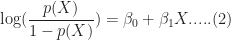
The quantity on the left is the logarithm of the odds. So, the model is a linear regression of the log-odds, sometimes called logit, and hence the name logistic.
The problem is to find the values of 

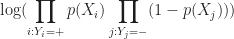
Where 
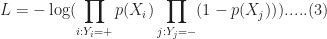
It should be noted that in practice one works with the log likelihood because it is easier to work with mathematically. Moreover, one minimises the negative log likelihood which, of course, is the same as maximising the log likelihood. The quantity one minimises is thus:
However, these are technical details that I mention only for completeness. As you will see next, they have little bearing on the practical use of logistic regression.
Logistic regression in R – an example
In this example, we’ll use the logistic regression option implemented within the glm function that comes with the base R installation. This function fits a class of models collectively known as generalized linear models. We’ll apply the function to the Pima Indian Diabetes dataset that comes with the mlbench package. The code is quite straightforward – particularly if you’ve read earlier articles in my “gentle introduction” series – so I’ll just list the code below noting that the logistic regression option is invoked by setting family=”binomial” in the glm function call.
Here we go:
Although this seems pretty good, we aren’t quite done because there is an issue that is lurking under the hood. To see this, let’s examine the information output from the model summary, in particular the coefficient estimates (i.e. estimates for 
- Column 2 in the table lists coefficient estimates.
- Column 3 list s the standard error of the estimates (the larger the standard error, the less confident we are about the estimate)
- Column 4 the z statistic (which is the coefficient estimate (column 2) divided by the standard error of the estimate (column 3)) and
- The last column (Pr(>|z|) lists the p-value, which is the probability of getting the listed estimate assuming the predictor has no effect. In essence, the smaller the p-value, the more significant the estimate is likely to be.
From the table we can conclude that only 4 predictors are significant – pregnant, glucose, mass and pedigree (and possibly a fifth – pressure). The other variables have little predictive power and worse, may contribute to overfitting. They should, therefore, be eliminated and we’ll do that in a minute. However, there’s an important point to note before we do so…
In this case we have only 9 variables, so are able to identify the significant ones by a manual inspection of p-values. As you can well imagine, such a process will quickly become tedious as the number of predictors increases. Wouldn’t it be be nice if there were an algorithm that could somehow automatically shrink the coefficients of these variables or (better!) set them to zero altogether? It turns out that this is precisely what lasso and its close cousin, ridge regression, do.
Ridge and Lasso
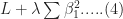
Recall that the values of the logistic regression coefficients 


and

Where 
In the case of ridge regression, the effect of the penalty term is to shrink the coefficients that contribute most to the error. Put another way, it reduces the magnitude of the coefficients that contribute to increasing 
Let’s illustrate this through an example. We’ll use the glmnet package which implements a combined version of ridge and lasso (called elastic net). Instead of minimising (4) or (5) above, glmnet minimises:
![L +\lambda[ (1-\alpha)\sum [\beta_1^2 + \alpha\sum|\beta_1|]....(6)](https://s0.wp.com/latex.php?latex=L+%2B%5Clambda%5B+%281-%5Calpha%29%5Csum+%5B%5Cbeta_1%5E2+%2B+%5Calpha%5Csum%7C%5Cbeta_1%7C%5D....%286%29&bg=ffffff&fg=1c1c1c&s=0&c=20201002)
where 


Lasso regularisation using glmnet
Let’s reanalyse the Pima Indian Diabetes dataset using glmnet with
- does not have a formula interface, so one has to input the predictors as a matrix and the class labels as a vector.
- does not accept categorical predictors, so one has to convert these to numeric values before passing them to glmnet.
The glmnet function model.matrix creates the matrix and also converts categorical predictors to appropriate dummy variables.
Another important point to note is that we’ll use the function cv.glmnet, which automatically performs a grid search to find the optimal value of
OK, enough said, here we go:
The plot is shown in Figure 2 below:

Figure 2: Error as a function of lambda (select lambda that minimises error)
The plot shows that the log of the optimal value of lambda (i.e. the one that minimises the root mean square error) is approximately -5. The exact value can be viewed by examining the variable lambda_min in the code below. In general though, the objective of regularisation is to balance accuracy and simplicity. In the present context, this means a model with the smallest number of coefficients that also gives a good accuracy. To this end, the cv.glmnet function finds the value of lambda that gives the simplest model but also lies within one standard error of the optimal value of lambda. This value of lambda (lambda.1se) is what we’ll use in the rest of the computation. Interested readers should have a look at this article for more on lambda.1se vs lambda.min.
The output shows that only those variables that we had determined to be significant on the basis of p-values have non-zero coefficients. The coefficients of all other variables have been set to zero by the algorithm! Lasso has reduced the complexity of the fitting function massively…and you are no doubt wondering what effect this has on accuracy. Let’s see by running the model against our test data:
Which is a bit less than what we got with the more complex model. So, we get a similar out-of-sample accuracy as we did before, and we do so using a way simpler function (4 non-zero coefficients) than the original one (9 nonzero coefficients). What this means is that the simpler function does at least as good a job fitting the signal in the data as the more complicated one. The bias-variance tradeoff tells us that the simpler function should be preferred because it is less likely to overfit the training data.
Paraphrasing William of Ockham: all other things being equal, a simple hypothesis should be preferred over a complex one.
Wrapping up
In this post I have tried to provide a detailed introduction to logistic regression, one of the simplest (and oldest) classification techniques in the machine learning practitioners arsenal. Despite it’s simplicity (or I should say, because of it!) logistic regression works well for many business applications which often have a simple decision boundary. Moreover, because of its simplicity it is less prone to overfitting than flexible methods such as decision trees. Further, as we have shown, variables that contribute to overfitting can be eliminated using lasso (or ridge) regularisation, without compromising out-of-sample accuracy. Given these advantages and its inherent simplicity, it isn’t surprising that logistic regression remains a workhorse for data scientists.


[…] In this day and age of artificial intelligence and deep learning, it is easy to forget that simple algorithms can work well for a surprisingly large range of practical business problems. And the simplest place to start is with the granddaddy of data science algorithms: linear regression and its close… Read more: A gentle introduction to logistic regression and lasso regularisation using R […]
LikeLike
A gentle introduction to logistic regression and lasso regularisation using R – Best Project Management Aggregators
July 12, 2017 at 11:35 am
Hi, Kailash
Thanks for informative post.
One remark concerning Occam’s Razor and machine learning – it is not so unambiguous – have a look at the work of Geoff Webb – http://i.giwebb.com/index.php/research/occams-razor-in-machine-learning/
Kind Regards
Serhiy
LikeLiked by 1 person
Serhiy Yevtushenko
July 15, 2017 at 2:20 pm
good implementation, but I found one serious mistake. the second accuracy you obtained from lasso regression is lambda with 1se, not minimum. you should be getting accuracy of 70% by right.
LikeLike
youngseok jeon
September 11, 2017 at 6:13 pm
sorry I wrote wrong. the accuracy is for lambda with minumum. but the coeffs are for lambda with 1se.
LikeLike
youngseok jeon
September 11, 2017 at 6:17 pm
Hi Youngseok,
Many thanks for pointing this out, you’re absolutely right. I have fixed this in the code and have added a bit of discussion around lambda.1se vs lambda.min.
Regards,
Kailash.
LikeLike
K
September 12, 2017 at 3:04 pm
I tried to repeat the code, but i get:
“Error in !se.fit : invalid argument type” – error, when i try to run:
lasso_prob <- predict.glm(glm_model,testset[,-typeColNum],s=”lambda_1se”,type=”response”)
And what is the purpose of line:
x_test <- model.matrix(diabetes~.,testset)
because variable x_test isn't used anywhere. (Or at least i can't find anywhere)
LikeLike
Raimo Haikari
September 16, 2017 at 5:06 am
Hi Raimo,
Thanks so much for pointing this out. I had used the incorrect predict function (the one for glm instead of glmnet). This has now been fixed. I’ve run the code from start to end in a clean environment and seems all good now. Please do let me know if you encounter any issues.
Thanks again, I truly appreciate it.
Regards,
Kailash.
LikeLike
K
September 16, 2017 at 9:13 am
Any advice on extended this for non-binary classification? I’m trying to use Logistic regression for a 3 class data set and am having very little success
LikeLike
Anna Ahern
October 6, 2017 at 1:51 am
Hi Anna,
This should be possible (though I have not tried it myself). See the section on Multinomial Models on page 23 of the glmnet vignette by Trevor Hastie: https://web.stanford.edu/~hastie/Papers/Glmnet_Vignette.pdf
Hope this helps.
Regards,
Kailash.
LikeLike
K
October 6, 2017 at 11:35 am
Great post! I was just wondering if you use type =”response” as your logistic regression loss function measurement, why not use something similar in LASSO implementation. e.g use type =”link” or type = “response”, given that this post is about logistic regression and MSE is really not an ideal loss function for logistic regression.
LikeLike
Jenny
October 26, 2017 at 12:58 am
Agree with Jenny, “deviance” should be a better loss in this case.
LikeLike
LazyBoo
January 11, 2018 at 9:20 am