An introduction to Monte Carlo simulation of project tasks
Introduction
In an essay on the uncertainty of project task estimates, I described how a task estimate corresponds to a probability distribution. Put simply, a task estimate is actually a range of possible completion times, each with a probability of occurrence specified by a distribution. If one knows the distribution, it is possible to answer questions such as: “What is the probability that the task will be completed within x days?”
The reliability of such predictions depends on how faithfully the distribution captures the actual spread of task durations – and therein lie at least a couple of problems. First, the probability distributions for task durations are generally hard to characterise because of the lack of reliable data (estimators are not very good at estimating, and historical data is usually not available). Second, many realistic distributions have complicated mathematical forms which can be hard to characterise and manipulate.
These problems are compounded by the fact that projects consist of several tasks, each one with its own duration estimate and (possibly complicated) distribution. The first issue is usually addressed by fitting distributions to point estimates (such as optimistic, pessimistic and most likely times as in PERT) and then refining these estimates and distributions as one gains experience. The second issue can be tackled by Monte Carlo techniques, which involve simulating the task a number of times (using an appropriate distribution) and then calculating expected completion times based on the results. My aim in this post is to present an example-based introduction to Monte Carlo simulation of project task durations.
Although my aim is to keep things reasonably simple (not too much beyond high-school maths and a basic understanding of probability), I’ll be covering a fair bit of ground. Given this, I’d best to start with a brief description of my approach so that my readers know what coming.
Monte Carlo simulation is an umbrella term that covers a range of approaches that use random sampling to simulate events that are described by known probability distributions. The first task then, is to specify the probability distribution. However, as mentioned earlier, this is generally unknown for task durations. For simplicity, I’ll assume that task duration uncertainty can be described accurately using a triangular probability distribution – a distribution that is particularly easy to handle from the mathematical point of view. The advantage of using the triangular distribution is that simulation results can be validated easily.
Using the triangular distribution isn’t a limitation because the method I describe can be applied to arbitrarily shaped distributions. More important, the technique can be used to simulate what happens when multiple tasks are strung together as in a project schedule (I’ll cover this in a future post). Finally, I’ll demonstrate a Monte Carlo simulation method as applied to a single task described by a triangular distribution. Although a simulation is overkill in this case (because questions regarding durations can be answered exactly without using a simulation), the example serves to illustrate the steps involved in simulating more complex cases – such as those comprising of more than one task and/or involving more complicated distributions.
So, without further ado, let me begin the journey by describing the triangular distribution.
The triangular distribution
Let’s assume that there’s a project task that needs doing, and the person who is going to do it reckons it will take between 2 and 8 hours to complete it, with a most likely completion time of 4 hours. How the estimator comes up with these numbers isn’t important at this stage – maybe there’s some guesswork, maybe some padding or maybe it is really based on experience (as it should be). What’s important is that we have three numbers corresponding to a minimum, most likely and maximum time. To keep the discussion general, we’ll call these 


Now, what about the probabilities associated with each of these times?
Since 


Figure 1: Triangular Distribution
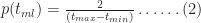
For the simulation, we need to know the equation describing the above distribution. Although Wikipedia will tell us the answer in a mouse-click, it is instructive to figure it out for ourselves. First, note that the area under the triangle must be equal to 1 because the task must finish at some time between

where 
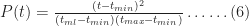
To derive the probability for any time
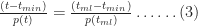
This is a consequence of the fact that the ratios on either side of equation (3) are equal to the slope of the line joining the points 


Figure 2
Substituting (2) in (3) and simplifying a bit, we obtain:
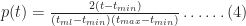

In a similar fashion one can show that the probability for times lying between
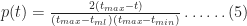

Equations 4 and 5 together describe the probability distribution function (or PDF) for all times between
Another quantity of interest is the cumulative distribution function (or CDF) which is the probability, 


Noting that for 

As expected,
To end this section let's plug in the numbers quoted by our estimator at the start of this section: 


Figure 4 – Triangular CDF (tmin=2, tml=4, tmax=8)
Monte Carlo Simulation of a Single Task
OK, so now we get to the business end of this essay – the simulation. I’ll first outline the simulation procedure and then discuss results for the case of the task described in the previous section (triangular distribution with
So, here’s my simulation procedure:
- Generate a random number between 0 and 1. Treat this number as the cumulative probability,
- Find the time,
- Repeat steps (1) and (2) N times, where N is a “sufficiently large” number – say 10,000.
I did the calculations for 
As an example of a simulation run proceeds, here’s the data from my first simulation run: the random number generator returned 0.490474700804856 (call it 0.4905). This is the value of 

Figure 5
After completing 10,000 simulation runs, I sorted these into bins corresponding to time intervals of .25 hrs, starting from

Figure 6: Distribution of simulation runs
As one might expect, this looks like the triangular distribution shown in Figure 4. There is a difference though: Figure 4 plots probability as a continuous function of time whereas Figure 6 plots the number of simulation runs as a step function of time. To convince ourselves that the two are really the same, lets look at the cumulative probability at 

Wrap up
A limitation of the triangular distribution is that it imposes an upper cut-off at
Another point worth mentioning is that simulations can be done at a level higher than that of an indivdual task. In their brilliant book – Waltzing With Bears: Managing Risk on Software Projects – De Marco and Lister demonstrate the use of Monte Carlo methods to simulate various aspects of project – velocity, time, cost etc. – at the project level (as opposed to the task level). I believe it is better to perform simulations at the lowest possible level (although it is a lot more work) – the main reason being that it is easier, and less error-prone, to estimate individual tasks than entire projects. Nevertheless, high level simulations can be very useful if one has reliable data to base these on.
I would be remiss if I didn’t mention some of the various Monte Carlo packages available in the market. I’ve never used any of these, but by all accounts they’re pretty good: see this commercial package or this one, for example. Both products use random number generators and sampling techniques that are far more sophisticated than the simple ones I’ve used in my example.
Finally, I have to admit that the example described in this post is a very complicated way of demonstrating the obvious – I started out with the triangular distribution and then got back the triangular distribution via simulation. My point, however, was to illustrate the method and show that it yields expected results in a situation where the answer is known. In a future post I’ll apply the method to more complex situations- for example, multiple tasks in series and parallel, with some dependency rules thrown in for good measure. Although, I’ll use the triangular distribution for individual tasks, the results will be far from obvious: simulation methods really start to shine as complexity increases. But all that will have to wait for later. For now, I hope my example has helped illustrate how Monte Carlo methods can be used to simulate project tasks.
Note added on 21 Sept 2009:
Follow-up to this article published here.
Note added on 14 Dec 2009:
See this post for a Monte Carlo simulation of correlated project tasks.


[…] An introduction to Monte Carlo simulation of project tasks « Eight to Late (tags: simulation project-management prediction) […]
LikeLike
links for 2009-09-11 « Blarney Fellow
September 12, 2009 at 12:35 pm
Hi Kailash,
Brilliant post and an great example to help us understand. But the only concern is the 3 point estimates (PERT). In an earlier post you had provided us links to a RAND corporation link about how PERT was a commercial makeover by the US DoD. PERT has several problems like “Merge Bias”, focussing only on critical path, neglecting correlation coefficients etc.. How do you still think 3 point estimates are a good start for Monte Carlo analysis? Will the final results from the simulation not have these as well?
LikeLike
Prakash
September 14, 2009 at 3:10 am
Prakash,
That’s an excellent point – and one that I should’ve explained in the post.
Anyway, here goes:
First, PERT – as it is commonly used- calculates expected task durations (typically via 3 point estimates) and then treats these as deterministic – i.e. the expected (or average) duration is treated as the task duration. This is OK for single tasks, as long as one understands that one is looking at the average completion time (over several trials). However, when one chains several tasks together, as in a project , it is no longer true that expected values add up (except in special cases). This point will be made clear in my next post on the topic, where I will deal with the simulation of multiple tasks (actually, only 2 tasks – but that will be enough to illustrate my point).
Second, the method described above is actually more realistic than a simple PERT treatment because the output is a range of possible completion times – each with a probability attached to it. Consequently, one can answer questions such as: “What is the probability of completion by time t?”. Now, of course, this question can be answered straight off (without simulation) for a single task described by a triangular distribution, but is well nigh impossible to answer straight-off for multiple tasks. Simulation is the only way for the latter.
Third, when simulating multiple tasks one can add in realistic inter-task events – such as delays etc. The merge path problem you mention is a consequence of ignoring slack path contributions to schedule risk. Simulations can take these into consideration as a matter of course.
Finally, as I’ve mentioned in the post, I’ve used the triangular distribution for illustrative purposes – the method described can be applied to any distribution.
Hope this addresses your question – do let me know if it doesn’t. Thanks again for raising an excellent point!
Regards,
Kailash.
LikeLike
K
September 14, 2009 at 5:57 am
[…] my previous post I demonstrated the use of a Monte Carlo technique in simulating a single project task with […]
LikeLike
Monte Carlo simulation of multiple project tasks – three examples and some general comments « Eight to Late
September 20, 2009 at 9:36 pm
[…] use of Monte Carlo simulations in project management (Note added on 23 Nov 2009: See my post on Monte Carlo simulations of project task durations for a quick introduction to the […]
LikeLike
An introduction to the critical chain method « Eight to Late
November 23, 2009 at 9:54 pm
[…] time ago, I wrote a couple of posts on Monte Carlo simulation of project tasks: the the first post presented a fairly detailed introduction to the technique and the second illustrated its use via […]
LikeLike
The effect of task duration correlations on project uncertainty – a study using Monte Carlo simulation « Eight to Late
December 11, 2009 at 10:00 am
[…] This post was mentioned on Twitter by Cornelius Fichtner and Vladimir Fadeev, Torsten J. Koerting. Torsten J. Koerting said: Easy to understand => An introduction to Monte Carlo simulation of project tasks by Eight to Late http://bit.ly/3gfM83 /via @corneliusficht […]
LikeLike
Tweets that mention An introduction to Monte Carlo simulation of project tasks « Eight to Late -- Topsy.com
December 15, 2009 at 9:11 am
[…] aren’t hard to follow – and I take the opportunity to plug my article entitled An introduction to Monte Carlo simulations of project tasks . As far as practice is concerned, there are several commercially available tools that […]
LikeLike
The failure of risk management: a book review « Eight to Late
February 11, 2010 at 10:13 pm
[…] their way into project management practice, albeit gradually. A good example of this is the use of Monte Carlo methods to estimate project variables. Such tools enable the project manager to present estimates in terms of probabilities (e.g. […]
LikeLike
Bayes Theorem for project managers « Eight to Late
March 11, 2010 at 10:17 pm
[…] which tells us not to put all our money on one horse, or eggs in one basket etc. See my introductory post on Monte Carlo simulations to see an example of how multiple uncertain quantities can combine in different […]
LikeLike
The Flaw of Averages – a book review « Eight to Late
May 4, 2010 at 11:06 pm
[…] of great practical importance because of the increasing use of probabilistic techniques (such as Monte Carlo methods) in decision making. Those who advocate the use of these methods generally assume that […]
LikeLike
On the interpretation of probabilities in project management « Eight to Late
July 1, 2010 at 10:09 pm
[…] of uncertainty can be combined via Monte Carlo simulation. Readers may find it helpful to keep my introduction to Monte Carlo simulations of project tasks handy, as I refer to it extensively in the present […]
LikeLike
Monte Carlo simulation of risk and uncertainty in project tasks | Eight to Late
February 17, 2011 at 9:56 pm
[…] used in developing estimates; indeed there are a good number of articles on this blog – see this post or this one, for example. However, most of these writings focus on the practical applications of […]
LikeLike
The shape of things to come: an essay on probability in project estimation « Eight to Late
April 3, 2012 at 11:40 pm
[…] deployed all the dark arts of simulations and Gantt Charts. All to no avail, my project will fail; I may as well be throwing […]
LikeLike
A project management dilemma in five limericks « Eight to Late
July 28, 2012 at 11:58 am
[…] above is that quantifiable uncertainties are shapes rather than single numbers. See this post and this one for details for how far this kind of reasoning can take you. That said, one should always be […]
LikeLike
Uncertainty, ambiguity and the art of decision making | Eight to Late
March 9, 2017 at 10:04 am